Take Home Assignment 3

Introduction

I picked MC3 of VAST Challenge 2024. The objective of the exercise is to help help FishEye to better identify bias, track behavior changes, and infer temporal patterns from the knowledge graphs prepared by their data analysts.

We will focus on task 1 in the mini-challenge, which is:

1. FishEye analysts want to better visualize changes in corporate structures over time. Create a visual analytics approach that analysts can use to highlight temporal patterns and changes in corporate structures. Examine the most active people and businesses using visual analytics.

Data Preparation

Load library and data

Show code

pacman::p_load(jsonlite, tidygraph, ggraph, visNetwork, graphlayouts, ggforce, skimr, tidytext, tidyverse, RColorBrewer) 
options(warn=-1)

json_text <- readLines("data/mc3.json")
json_text_fixed <- gsub("NaN", "null", json_text)
writeLines(json_text_fixed, "data/mc3_fixed.json")
mc3_data <- fromJSON("data/mc3_fixed.json")

Nodes and Edges overview

Nodes

Show code

mc3_nodes <- as_tibble(mc3_data$nodes)
glimpse(mc3_nodes)

Rows: 60,520
Columns: 15
$ type                <chr> "Entity.Organization.Company", "Entity.Organizatio…
$ country             <chr> "Uziland", "Mawalara", "Uzifrica", "Islavaragon", …
$ ProductServices     <chr> "Unknown", "Furniture and home accessories", "Food…
$ PointOfContact      <chr> "Rebecca Lewis", "Michael Lopez", "Steven Robertso…
$ HeadOfOrg           <chr> "Émilie-Susan Benoit", "Honoré Lemoine", "Jules La…
$ founding_date       <chr> "1954-04-24T00:00:00", "2009-06-12T00:00:00", "202…
$ revenue             <dbl> 5994.73, 71766.67, 0.00, 0.00, 4746.67, 46566.67, …
$ TradeDescription    <chr> "Unknown", "Abbott-Gomez is a leading manufacturer…
$ `_last_edited_by`   <chr> "Pelagia Alethea Mordoch", "Pelagia Alethea Mordoc…
$ `_last_edited_date` <chr> "2035-01-01T00:00:00", "2035-01-01T00:00:00", "203…
$ `_date_added`       <chr> "2035-01-01T00:00:00", "2035-01-01T00:00:00", "203…
$ `_raw_source`       <chr> "Existing Corporate Structure Data", "Existing Cor…
$ `_algorithm`        <chr> "Automatic Import", "Automatic Import", "Automatic…
$ id                  <chr> "Abbott, Mcbride and Edwards", "Abbott-Gomez", "Ab…
$ dob                 <chr> NA, NA, NA, NA, NA, NA, NA, NA, NA, NA, NA, NA, NA…

Only type, and id are selected.

Show code

mc3_nodes <- as_tibble(mc3_data$nodes) %>%
  mutate(id=as.character(id), 
         type=as.character(type)) %>%
  select(id, type)

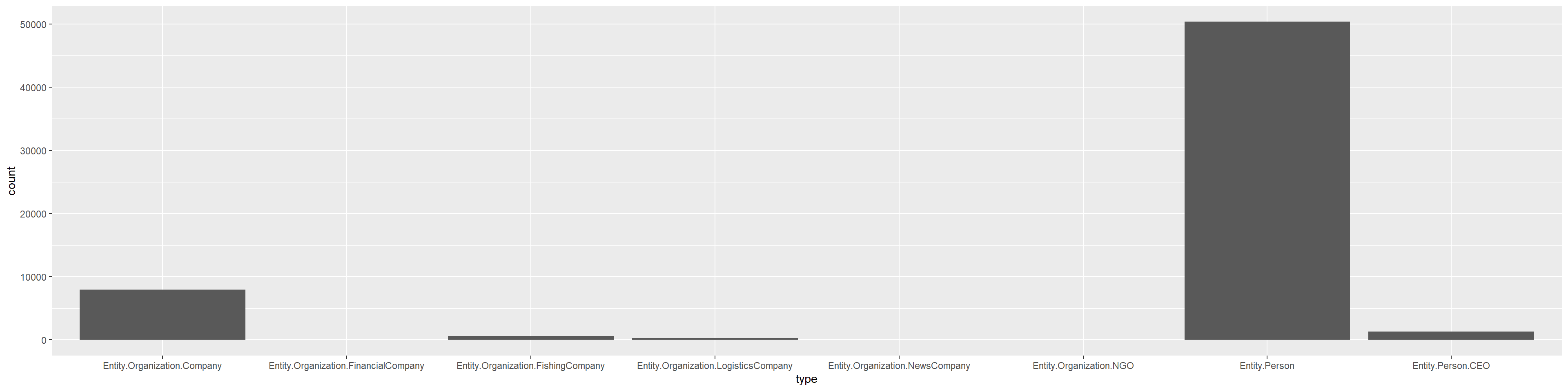
Below is the distribution of type column in nodes. It indicates that most entities are person, with some companies and CEOs. Other entities are negligible.

mc3_nodes$type %>% unique()

[1] "Entity.Organization.Company"         
[2] "Entity.Organization.LogisticsCompany"
[3] "Entity.Organization.FishingCompany"  
[4] "Entity.Organization.FinancialCompany"
[5] "Entity.Organization.NewsCompany"     
[6] "Entity.Organization.NGO"             
[7] "Entity.Person"                       
[8] "Entity.Person.CEO"                   

Edges

Show code

mc3_edges <- as_tibble(mc3_data$links)
head(mc3_edges)

# A tibble: 6 × 11
  start_date          type   `_last_edited_by` `_last_edited_date` `_date_added`
  <chr>               <chr>  <chr>             <chr>               <chr>        
1 2016-10-29T00:00:00 Event… Pelagia Alethea … 2035-01-01T00:00:00 2035-01-01T0…
2 2035-06-03T00:00:00 Event… Niklaus Oberon    2035-07-15T00:00:00 2035-07-15T0…
3 2028-11-20T00:00:00 Event… Pelagia Alethea … 2035-01-01T00:00:00 2035-01-01T0…
4 2024-09-04T00:00:00 Event… Pelagia Alethea … 2035-01-01T00:00:00 2035-01-01T0…
5 2034-11-12T00:00:00 Event… Pelagia Alethea … 2035-01-01T00:00:00 2035-01-01T0…
6 2007-04-06T00:00:00 Event… Pelagia Alethea … 2035-01-01T00:00:00 2035-01-01T0…
# ℹ 6 more variables: `_raw_source` <chr>, `_algorithm` <chr>, source <chr>,
#   target <chr>, key <int>, end_date <chr>

Show code

mc3_edges <- as_tibble(mc3_data$links) %>%
  distinct() %>%
  mutate(source = as.character(source), target=as.character(target), 
         type = as.character(type),  start_date=as.Date(start_date), 
         end_date=as.Date(end_date)) %>%
  select(type, source, target, start_date, end_date) %>%
  group_by(source, target, type) %>% 
  summarise(weights = n()) %>% 
  filter(source != target) %>%
  ungroup()

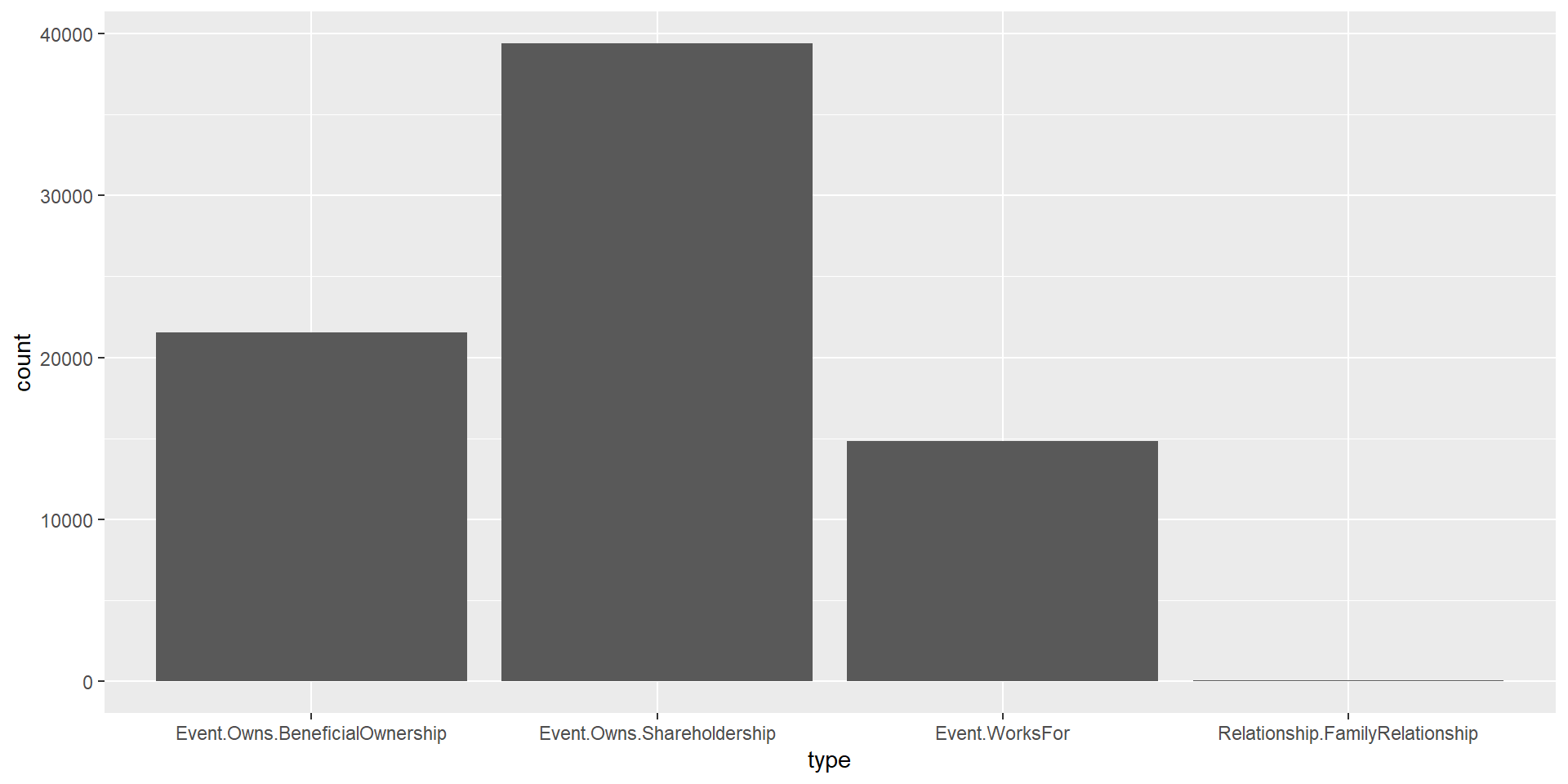
Below is the distribution of Type column in edges. It indicates that family relationship is negligible.

Show code

mc3_edges$type %>% unique()

[1] "Event.Owns.Shareholdership"      "Event.WorksFor"                 
[3] "Event.Owns.BeneficialOwnership"  "Relationship.FamilyRelationship"

Graph

Start with the entity with highest number. Sharon Moon

Show code

mc3_graph <- tbl_graph(nodes = mc3_nodes,
                       edges = mc3_edges,
                       directed = FALSE) %>% 
  mutate(betweenness_centrality = centrality_betweenness(), 
         closeness_centrality=centrality_closeness())

Show code

display_graph <- function() {
  # extract node with highest betweenness centrality
  top1_betw <- mc3_graph %>% 
    activate(nodes) %>% 
    as_tibble() %>% 
    top_n(1, betweenness_centrality) %>% 
      select(id, type)
  
  # extract lvl 1 edges
  top1_betw_edges_lvl1 <- mc3_edges %>% 
    filter(source %in% top1_betw[["id"]] | target %in% top1_betw[["id"]])
  
  # extract nodes from lvl 1 edges
  id1 <- top1_betw_edges_lvl1 %>%
    select(source) %>%
    rename(id = source) %>% 
    left_join(mc3_nodes, by = "id") %>% 
    select(id, type)
  
  id2 <- top1_betw_edges_lvl1 %>%
    select(target) %>%
    rename(id = target) %>% 
    left_join(mc3_nodes, by = "id") %>% 
    select(id, type)
  
  additional_nodes_lvl1 <- rbind(id1, id2) %>% 
    distinct %>% 
    filter(!id %in% top1_betw[["id"]])
  
  # extract lvl 2 edges
  top1_betw_edges_lvl2 <- mc3_edges %>% 
    filter(source %in% additional_nodes_lvl1[["id"]] | target %in% additional_nodes_lvl1[["id"]])
  
  # extract nodes from lvl 1 edges
  id1 <- top1_betw_edges_lvl2 %>%
    select(source) %>%
    rename(id = source) %>% 
    left_join(mc3_nodes, by = "id") %>% 
    select(id, type)
  
  id2 <- top1_betw_edges_lvl2 %>%
    select(target) %>%
    rename(id = target) %>% 
    left_join(mc3_nodes, by = "id") %>% 
    select(id, type)
  
  additional_nodes_lvl2 <- rbind(id1, id2) %>% 
    distinct %>% 
    filter(!id %in% top1_betw[["id"]] & !id %in% additional_nodes_lvl1[["id"]])
  
  # combine all nodes
  top1_betw_nodes <- rbind(top1_betw, additional_nodes_lvl1, additional_nodes_lvl2) %>%
    distinct()
  
  # combine all edges
  top1_betw_edges <- rbind(top1_betw_edges_lvl1, top1_betw_edges_lvl2) %>% 
    distinct()
  
  # colur palatte for betweenness centrality colours
  sw_colors <- colorRampPalette(brewer.pal(3, "RdBu"))(3)
  
  # customise edges for plotting
  top1_betw_edges <- top1_betw_edges %>% 
    rename(from = source,
           to = target) %>% 
    mutate(title = paste0("Type: ", type), # tooltip when hover over
           color = "#0085AF") # color of edge
  
  # customise nodes for plotting
  top1_betw_nodes <- top1_betw_nodes %>% 
    rename(group = type) %>% 
    mutate(id.type = ifelse(id == top1_betw[["id"]], sw_colors[1], sw_colors[2])) %>%
    mutate(title = paste0(id, "<br>Group: ", group), # tooltip when hover over
           size = 30, # set size of nodes
           color.border = "#013848", # border colour of nodes
           color.background = id.type, # background colour of nodes
           color.highlight.background = "#FF8000" # background colour of nodes when highlighted
           )

  # plot graph
  visNetwork(top1_betw_nodes, top1_betw_edges,
             height = "700px", width = "100%",
             main = paste0("Network Graph of ", top1_betw[["id"]])) %>%
    visIgraphLayout() %>%
    visGroups(groupname = "Entity.Organization.Company", shape = "triangle") %>%
    visGroups(groupname = "Entity.Organization.FishingCompany", shape = "triangle") %>%
    visGroups(groupname = "Entity.Person", shape = "circle") %>%  
    visGroups(groupname = "Entity.Person.CEO", shape = "circle") %>%  
    visOptions(selectedBy = "group",
               highlightNearest = list(enabled = T, degree = 1, hover = T),
               nodesIdSelection = FALSE) %>% 
    visLayout(randomSeed = 123)

}

display_graph()

Visualization With Time

Show code

mc3_edges <- as_tibble(mc3_data$links) %>%
  mutate(source = as.character(source), target=as.character(target), 
         type = as.character(type),  start_date=as.Date(start_date), 
         end_date=as.Date(end_date)) %>%
  select(type, source, target, start_date, end_date)

mc3_edges$year <- as.integer(format(mc3_edges$start_date, "%Y"))

The year range for start time of activity: 1952 to 2035

min(mc3_edges$year, na.rm=TRUE)

[1] 1952

max(mc3_edges$year, na.rm=TRUE)

[1] 2035

Show code

display_graph_with_time <- function(entity_id, end_year) {
  mc3_edges <- as_tibble(mc3_data$links) %>%
    mutate(source = as.character(source), target=as.character(target), 
           type = as.character(type),  start_date=as.Date(start_date), 
           end_date=as.Date(end_date)) %>%
    select(type, source, target, start_date, end_date)
    
  mc3_edges$year <- as.integer(format(mc3_edges$start_date, "%Y"))
  mc3_edges <- mc3_edges %>% 
    filter(year<=end_year) %>%
    group_by(source, target, type) %>% 
    summarise(weights = n()) %>% 
    filter(source != target) %>%
    ungroup()
  
  mc3_nodes <- mc3_nodes %>%
  filter(id %in% c(mc3_edges$source, mc3_edges$target))
  
  mc3_graph <- tbl_graph(nodes = mc3_nodes, edges = mc3_edges, directed = FALSE) %>% 
    mutate(betweenness_centrality = centrality_betweenness(), closeness_centrality=centrality_closeness())
  
  
  # extract node with highest betweenness centrality
  top1_betw <- mc3_nodes %>% 
    filter(id==entity_id)
  
  # extract lvl 1 edges
  top1_betw_edges_lvl1 <- mc3_edges %>% 
    filter(source %in% top1_betw[["id"]] | target %in% top1_betw[["id"]])
  
  # extract nodes from lvl 1 edges
  id1 <- top1_betw_edges_lvl1 %>%
    select(source) %>%
    rename(id = source) %>% 
    left_join(mc3_nodes, by = "id") %>% 
    select(id, type)
  
  id2 <- top1_betw_edges_lvl1 %>%
    select(target) %>%
    rename(id = target) %>% 
    left_join(mc3_nodes, by = "id") %>% 
    select(id, type)
  
  additional_nodes_lvl1 <- rbind(id1, id2) %>% 
    distinct %>% 
    filter(!id %in% top1_betw[["id"]])
  
  # extract lvl 2 edges
  top1_betw_edges_lvl2 <- mc3_edges %>% 
    filter(source %in% additional_nodes_lvl1[["id"]] | target %in% additional_nodes_lvl1[["id"]])
  
  # extract nodes from lvl 1 edges
  id1 <- top1_betw_edges_lvl2 %>%
    select(source) %>%
    rename(id = source) %>% 
    left_join(mc3_nodes, by = "id") %>% 
    select(id, type)
  
  id2 <- top1_betw_edges_lvl2 %>%
    select(target) %>%
    rename(id = target) %>% 
    left_join(mc3_nodes, by = "id") %>% 
    select(id, type)
  
  additional_nodes_lvl2 <- rbind(id1, id2) %>% 
    distinct %>% 
    filter(!id %in% top1_betw[["id"]] & !id %in% additional_nodes_lvl1[["id"]])
  
  # combine all nodes
  top1_betw_nodes <- rbind(top1_betw, additional_nodes_lvl1, additional_nodes_lvl2) %>%
    distinct()
  
  # combine all edges
  top1_betw_edges <- rbind(top1_betw_edges_lvl1, top1_betw_edges_lvl2) %>% 
    distinct()
  
  # colur palatte for betweenness centrality colours
  sw_colors <- colorRampPalette(brewer.pal(3, "RdBu"))(3)
  
  # customise edges for plotting
  top1_betw_edges <- top1_betw_edges %>% 
    rename(from = source,
           to = target) %>% 
    mutate(title = paste0("Type: ", type), # tooltip when hover over
           color = "#0085AF") # color of edge
  
  # customise nodes for plotting
  top1_betw_nodes <- top1_betw_nodes %>% 
    rename(group = type) %>% 
    mutate(id.type = ifelse(id == top1_betw[["id"]], sw_colors[1], sw_colors[2])) %>%
    mutate(title = paste0(id, "<br>Group: ", group), # tooltip when hover over
           size = 30, # set size of nodes
           color.border = "#013848", # border colour of nodes
           color.background = id.type, # background colour of nodes
           color.highlight.background = "#FF8000" # background colour of nodes when highlighted
           )
  
  visNetwork(top1_betw_nodes, top1_betw_edges,
           height = "700px", width = "100%",
           main = paste0("Network Graph of ", entity_id)) %>%
    visIgraphLayout() %>%
    visGroups(groupname = "Entity.Organization.Company", shape = "triangle") %>%
    visGroups(groupname = "Entity.Organization.FishingCompany", shape = "triangle") %>%
    visGroups(groupname = "Entity.Person", shape = "circle") %>%  
    visGroups(groupname = "Entity.Person.CEO", shape = "circle") %>%  
    visOptions(selectedBy = "group", highlightNearest = list(enabled = T, degree = 1, hover = T), nodesIdSelection = FALSE) %>% 
    visLayout(randomSeed = 123)
}

2020

display_graph_with_time('Sharon Moon', 2020)

`summarise()` has grouped output by 'source', 'target'. You can override using
the `.groups` argument.

2025

display_graph_with_time('Sharon Moon', 2025)

`summarise()` has grouped output by 'source', 'target'. You can override using
the `.groups` argument.

2030

display_graph_with_time('Sharon Moon', 2030)

`summarise()` has grouped output by 'source', 'target'. You can override using
the `.groups` argument.

2035

display_graph_with_time('Sharon Moon', 2035)

`summarise()` has grouped output by 'source', 'target'. You can override using
the `.groups` argument.

The display_graph_with_time(entity_id, year) provides a comprehensive way to visualize corporate structure over time. Due to the limitation of quarto, the visualization is not interactive enough, and could be improved further after migrating to shiny app with a time slider.

In general, the corporate structure for Sharon Moon expands quite significantly from 2020 to 2030. Besides, the related entities (level 1 and level 2 entities) also expands. However, the growing speed slows down after 2030, probably due to slower growth rate when reaching certain capacity, or the growth of the whole business slows down from 2030 to 2035.