pacman::p_load(sf, tmap, tidyverse)Hands-on 8
Choropleth Mapping
mpsz <- st_read(dsn = "../data/geospatial",
                layer = "MP14_SUBZONE_WEB_PL")
Reading layer `MP14_SUBZONE_WEB_PL' from data source
`C:\quarto\ISSS609-AY2023-24\isss608\data\geospatial' using driver `ESRI Shapefile'
Simple feature collection with 323 features and 15 fields
Geometry type: MULTIPOLYGON
Dimension: XY
Bounding box: xmin: 2667.538 ymin: 15748.72 xmax: 56396.44 ymax: 50256.33
Projected CRS: SVY21popdata <- read_csv("../data/aspatial/respopagesextod2011to2020.csv")Rows: 984656 Columns: 7
── Column specification ────────────────────────────────────────────────────────
Delimiter: ","
chr (5): PA, SZ, AG, Sex, TOD
dbl (2): Pop, Time
ℹ Use `spec()` to retrieve the full column specification for this data.
ℹ Specify the column types or set `show_col_types = FALSE` to quiet this message.popdata2020 <- popdata %>%
filter(Time == 2020) %>%
group_by(PA, SZ, AG) %>%
summarise(`POP` = sum(`Pop`)) %>%
ungroup() %>%
pivot_wider(names_from=AG,
values_from=POP) %>%
mutate(YOUNG = rowSums(.[3:6])
+rowSums(.[12])) %>%
mutate(`ECONOMY ACTIVE` = rowSums(.[7:11])+
rowSums(.[13:15]))%>%
mutate(`AGED`=rowSums(.[16:21])) %>%
mutate(`TOTAL`=rowSums(.[3:21])) %>%
mutate(`DEPENDENCY` = (`YOUNG` + `AGED`)
/`ECONOMY ACTIVE`) %>%
select(`PA`, `SZ`, `YOUNG`,
`ECONOMY ACTIVE`, `AGED`,
`TOTAL`, `DEPENDENCY`)`summarise()` has grouped output by 'PA', 'SZ'. You can override using the
`.groups` argument.popdata2020 <- popdata2020 %>%
mutate_at(.vars = vars(PA, SZ),
.funs = funs(toupper)) %>%
filter(`ECONOMY ACTIVE` > 0)Warning: `funs()` was deprecated in dplyr 0.8.0.
ℹ Please use a list of either functions or lambdas:
# Simple named list: list(mean = mean, median = median)
# Auto named with `tibble::lst()`: tibble::lst(mean, median)
# Using lambdas list(~ mean(., trim = .2), ~ median(., na.rm = TRUE))mpsz_pop2020 <- left_join(mpsz, popdata2020,
by = c("SUBZONE_N" = "SZ"))
write_rds(mpsz_pop2020, "../data/rds/mpszpop2020.rds")tmap_mode("plot")tmap mode set to plottingqtm(mpsz_pop2020,
fill = "DEPENDENCY")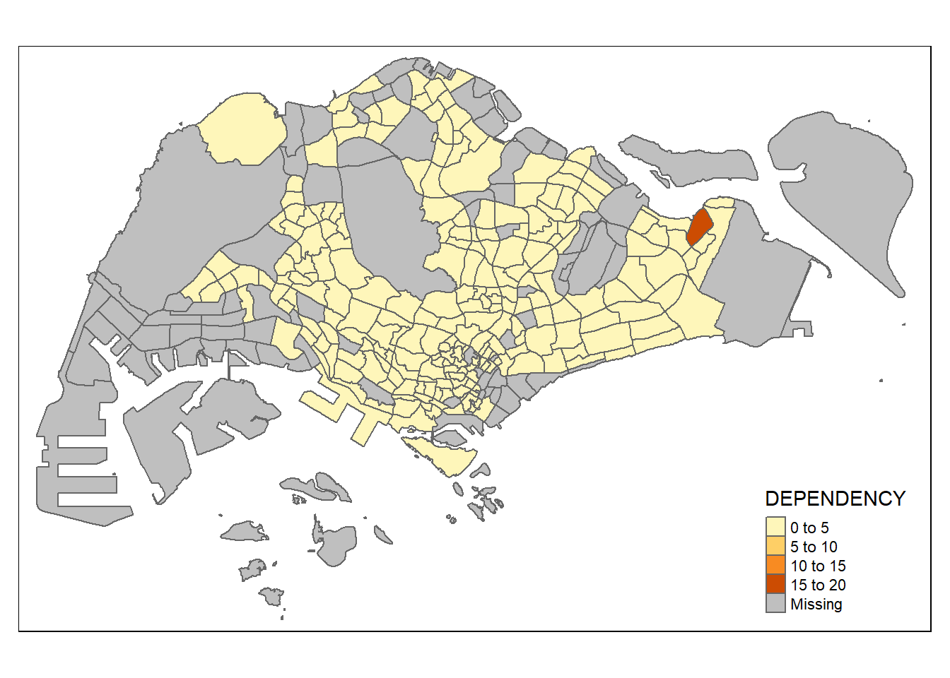
tm_shape(mpsz_pop2020)+
  tm_fill("DEPENDENCY",
          style = "quantile",
          palette = "Blues",
          title = "Dependency ratio") +
  tm_layout(main.title = "Distribution of Dependency Ratio by planning subzone",
            main.title.position = "center",
            main.title.size = 1.2,
            legend.height = 0.45,
            legend.width = 0.35,
            frame = TRUE) +
  tm_borders(alpha = 0.5) +
  tm_compass(type="8star", size = 2) +
  tm_scale_bar() +
  tm_grid(alpha =0.2) +
  tm_credits("Source: Planning Sub-zone boundary from Urban Redevelopment Authorithy (URA)\n and Population data from Department of Statistics DOS",
             position = c("left", "bottom"))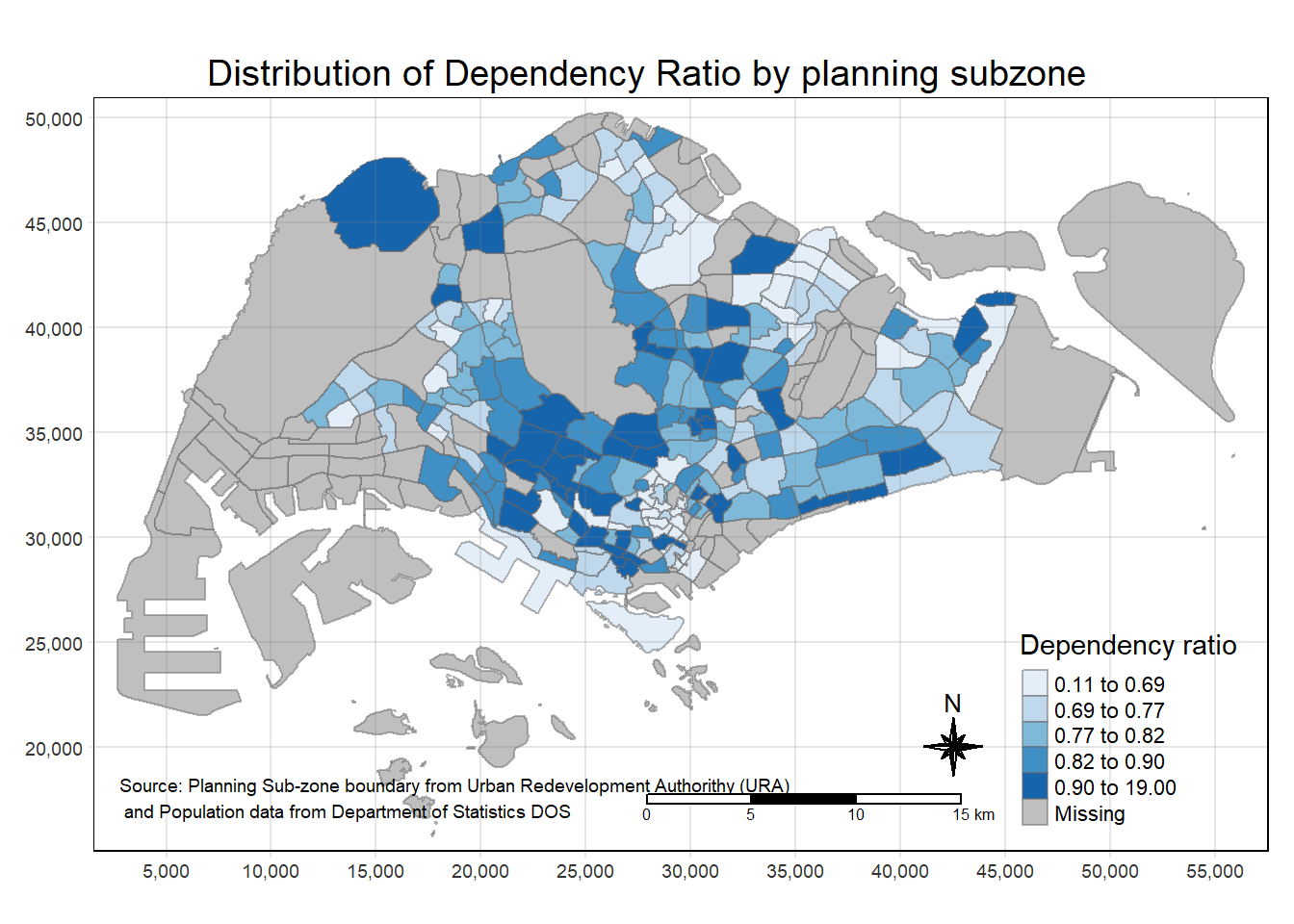
tm_shape(mpsz_pop2020)+
  tm_fill("DEPENDENCY")
tm_shape(mpsz_pop2020)+
  tm_fill("DEPENDENCY") +
  tm_borders(lwd = 0.1,  alpha = 1)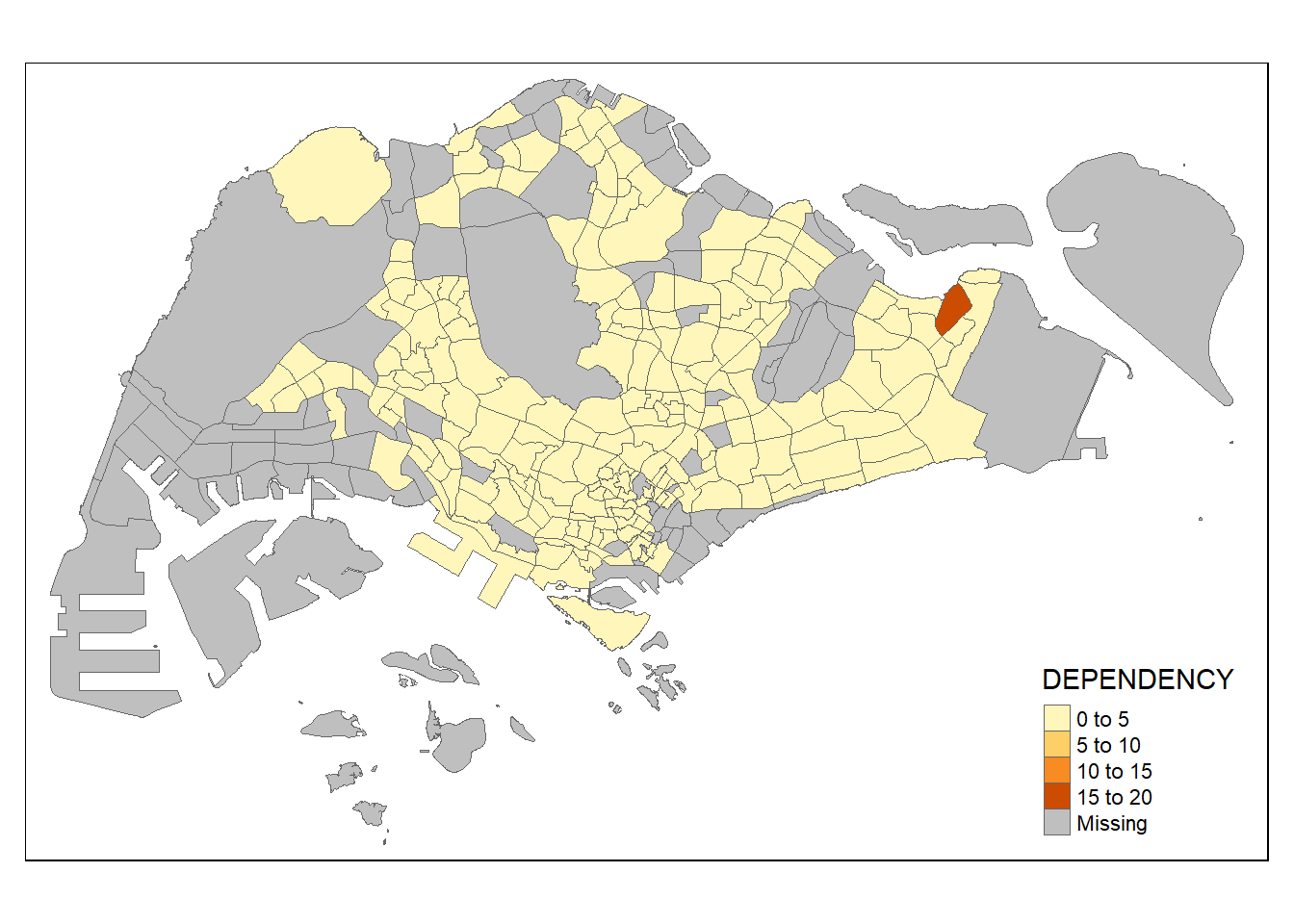
tm_shape(mpsz_pop2020)+
  tm_fill("DEPENDENCY",
          n = 5,
          style = "jenks") +
  tm_borders(alpha = 0.5)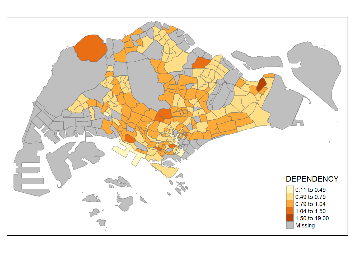
tm_shape(mpsz_pop2020)+
  tm_fill("DEPENDENCY",
          style = "quantile",
          palette = "Blues",
          title = "No. of persons") +
  tm_layout(main.title = "Distribution of Dependency Ratio \nby planning subzone",
            main.title.position = "center",
            main.title.size = 1.2,
            legend.height = 0.45,
            legend.width = 0.35,
            frame = TRUE) +
  tm_borders(alpha = 0.5) +
  tm_compass(type="8star", size = 2) +
  tm_scale_bar(width = 0.15) +
  tm_grid(lwd = 0.1, alpha = 0.2) +
  tm_credits("Source: Planning Sub-zone boundary from Urban Redevelopment Authorithy (URA)\n and Population data from Department of Statistics DOS",
             position = c("left", "bottom"))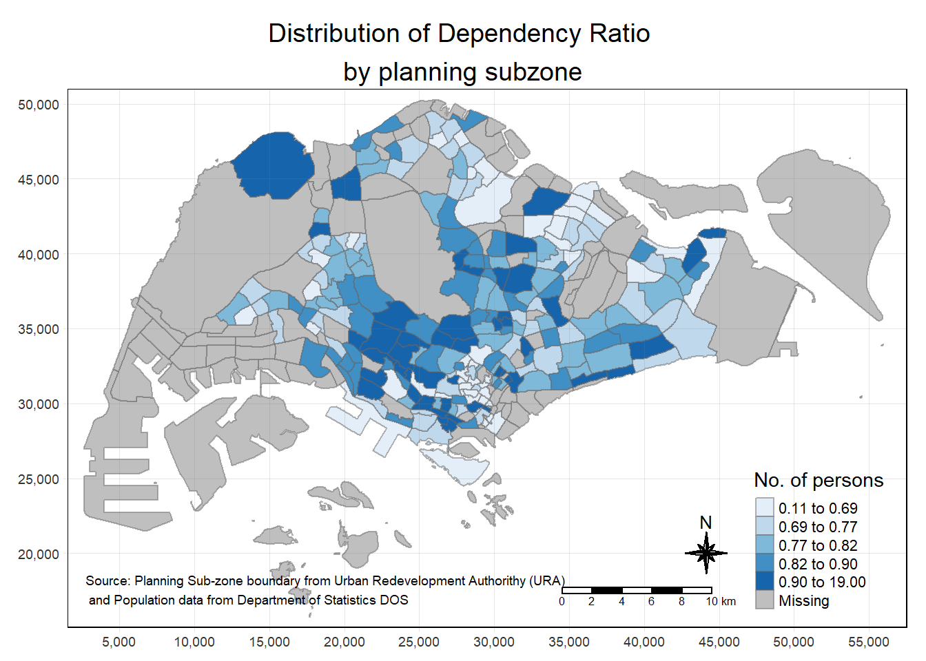
Reflection:
Display geographical info with different visualization options (color, style, etc.)
Visualising Geospatial Point Data
pacman::p_load(sf, tmap, tidyverse)sgpools <- read_csv("../data/aspatial/SGPools_svy21.csv")Rows: 306 Columns: 7
── Column specification ────────────────────────────────────────────────────────
Delimiter: ","
chr (3): NAME, ADDRESS, OUTLET TYPE
dbl (4): POSTCODE, XCOORD, YCOORD, Gp1Gp2 Winnings
ℹ Use `spec()` to retrieve the full column specification for this data.
ℹ Specify the column types or set `show_col_types = FALSE` to quiet this message.sgpools_sf <- st_as_sf(sgpools,
coords = c("XCOORD", "YCOORD"),
crs= 3414)
tmap_mode("view")tmap mode set to interactive viewingtm_shape(sgpools_sf)+
tm_bubbles(col = "red",
size = 1,
border.col = "black",
border.lwd = 1)tm_shape(sgpools_sf)+
tm_bubbles(col = "red",
size = "Gp1Gp2 Winnings",
border.col = "black",
border.lwd = 1)Legend for symbol sizes not available in view mode.tm_shape(sgpools_sf)+
tm_bubbles(col = "OUTLET TYPE",
size = "Gp1Gp2 Winnings",
border.col = "black",
border.lwd = 1)Legend for symbol sizes not available in view mode.tmap_mode("plot")tmap mode set to plottingAnalytical Mapping
pacman::p_load(tmap, tidyverse, sf)NGA_wp <- read_rds("../data/rds/NGA_wp.rds")p1 <- tm_shape(NGA_wp) +
tm_fill("wp_functional",
n = 10,
style = "equal",
palette = "Blues") +
tm_borders(lwd = 0.1,
alpha = 1) +
tm_layout(main.title = "Distribution of functional water point by LGAs",
legend.outside = FALSE)
p2 <- tm_shape(NGA_wp) +
tm_fill("total_wp",
n = 10,
style = "equal",
palette = "Blues") +
tm_borders(lwd = 0.1,
alpha = 1) +
tm_layout(main.title = "Distribution of total water point by LGAs",
legend.outside = FALSE)
tmap_arrange(p2, p1, nrow = 1)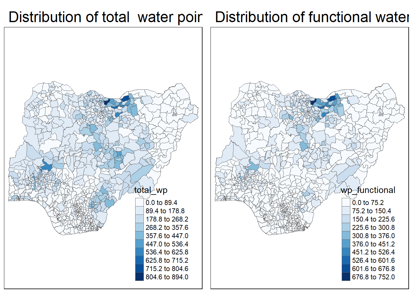
NGA_wp <- NGA_wp %>%
  mutate(pct_functional = wp_functional/total_wp) %>%
  mutate(pct_nonfunctional = wp_nonfunctional/total_wp)

tm_shape(NGA_wp) +
  tm_fill("pct_functional",
          n = 10,
          style = "equal",
          palette = "Blues",
          legend.hist = TRUE) +
  tm_borders(lwd = 0.1,
             alpha = 1) +
  tm_layout(main.title = "Rate map of functional water point by LGAs",
            legend.outside = TRUE)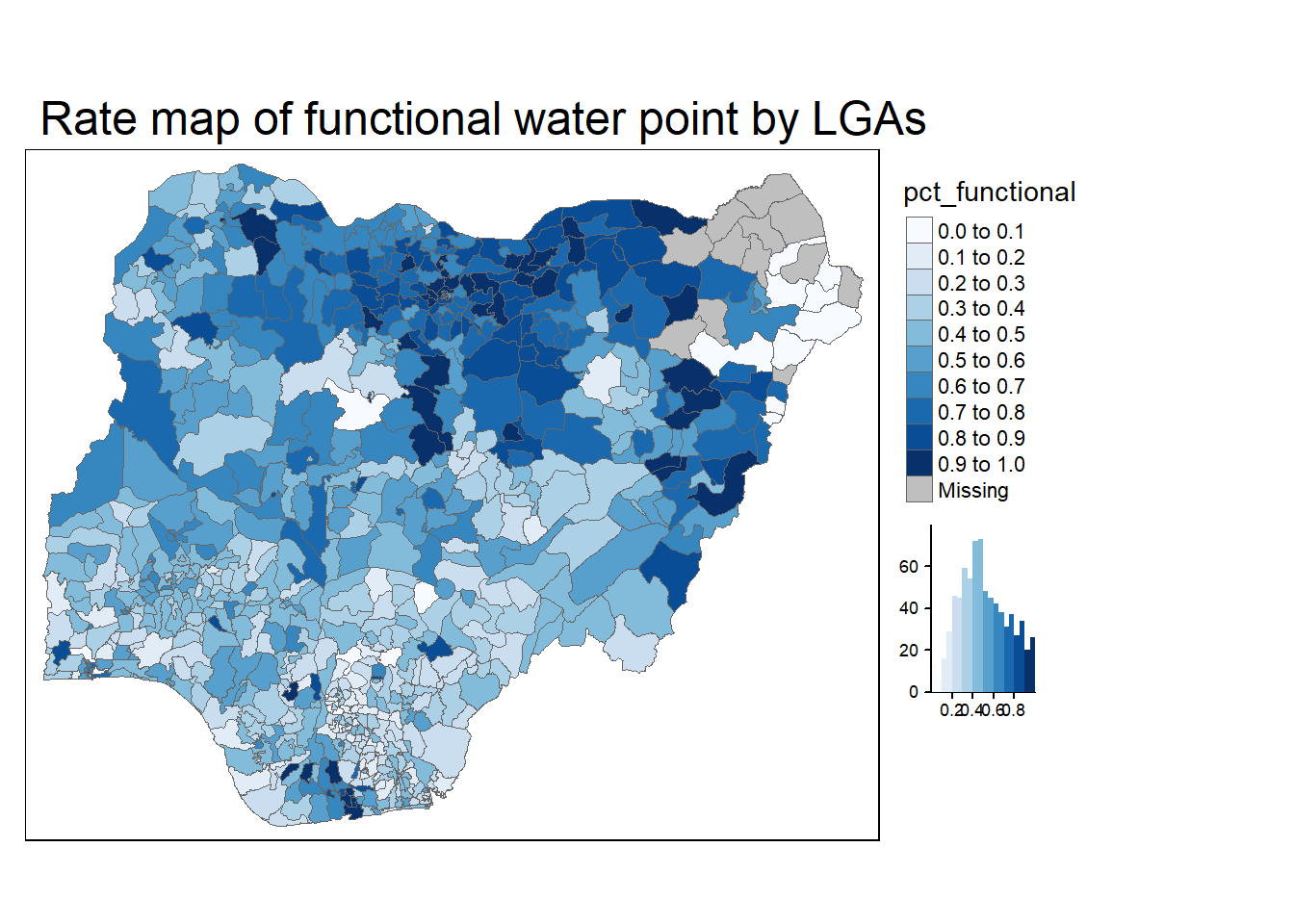
NGA_wp <- NGA_wp %>%
drop_na()
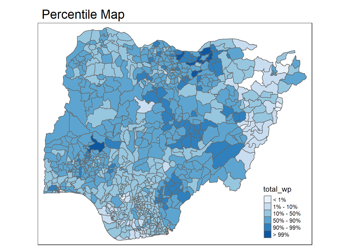
percent <- c(0,.01,.1,.5,.9,.99,1)
var <- NGA_wp["pct_functional"] %>%
st_set_geometry(NULL)
quantile(var[,1], percent) 0% 1% 10% 50% 90% 99% 100%
0.0000000 0.0000000 0.2169811 0.4791667 0.8611111 1.0000000 1.0000000 get.var <- function(vname,df) {
v <- df[vname] %>%
st_set_geometry(NULL)
v <- unname(v[,1])
return(v)
}
percentmap <- function(vnam, df, legtitle=NA, mtitle="Percentile Map"){
percent <- c(0,.01,.1,.5,.9,.99,1)
var <- get.var(vnam, df)
bperc <- quantile(var, percent)
tm_shape(df) +
tm_polygons() +
tm_shape(df) +
tm_fill(vnam,
title=legtitle,
breaks=bperc,
palette="Blues",
labels=c("< 1%", "1% - 10%", "10% - 50%", "50% - 90%", "90% - 99%", "> 99%")) +
tm_borders() +
tm_layout(main.title = mtitle,
title.position = c("right","bottom"))
}
percentmap("total_wp", NGA_wp)